Continuous diffusive measurement
Work in progress.
This tutorial is under construction, this is a draft version.
In this example, we simulate stochastic trajectories of quantum systems that are continuously measured by a diffusive detector. We explain how to use dq.dssesolve() to simulate trajectories modelled by the diffusive SSE, and dq.dsmesolve() to simulate trajectories modelled by the diffusive SME.
import jax
import jax.numpy as jnp
import numpy as np
from matplotlib import pyplot as plt
import dynamiqs as dq

dq.plot.mplstyle(dpi=150)  # set custom matplotlib style
Qubit
We consider a qubit starting from \(\ket{\psi_0}=\ket+_x=(\ket0+\ket1)/\sqrt2\), with no unitary dynamic \(H=0\) and a single loss operator \(L=\sigma_z\) which is continuously measured by a diffusive detector. We expect stochastic trajectories to project the qubit onto either of the \(\sigma_z\) eigenstates.
Let's begin with a perfectly efficient detector. We start with a pure state, and we measure all loss channels with perfect efficiency, so we don't loose any information about the system's state. As a result, it remains pure at all times. We use dq.dssesolve() to simulate these quantum trajectories.
Simulation
# define Hamiltonian, jump operators, initial state
H = dq.zeros(2)
jump_ops = [dq.sigmaz()]
psi0 = (dq.ground() + dq.excited()).unit()

# define save times
tsave = np.linspace(0, 1.0, 101)
delta_t = tsave[1] - tsave[0]

# define a certain number of PRNG key, one for each trajectory
key = jax.random.PRNGKey(20)
ntrajs = 5
keys = jax.random.split(key, ntrajs)

# simulate trajectories
method = dq.method.EulerMaruyama(dt=1e-3)
result = dq.dssesolve(H, jump_ops, psi0, tsave, keys, method=method)
print(result)
==== DSSESolveResult ====
Method       : EulerMaruyama
Infos        : 1000 steps | infos shape (5,)
States       : QArray complex64 (5, 101, 2, 1) | 7.9 Kb
Measurements : Array float32 (5, 1, 100) | 2.0 Kb
>>> result.states.shape  # (ntrajs, ntsave, n, 1)
(5, 101, 2, 1)
>>> result.measurements.shape  # (ntrajs, nLm, ntsave-1)
(5, 1, 100)
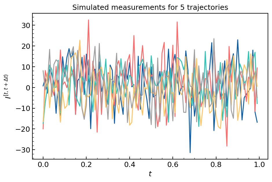
Individual trajectories
Iks = result.measurements[:, 0]
for Ik in Iks:
    plt.plot(tsave[:-1], Ik, lw=1.5)

plt.gca().set(
    title=rf'Simulated measurements for 5 trajectories',
    xlabel=r'$t$',
    ylabel=r'$I^{[t,t+\Delta t)}$',
)
Cumulative measurements
for Ik in Iks:
    cumsum_Ik = jnp.cumsum(Ik)
    plt.plot(tsave[1:], cumsum_Ik, lw=1.5)

plt.axhline(0, ls='--', lw=1.0, color='gray')
plt.gca().set(
    title=r'Integral of the measurement record',
    xlabel=r'$t$',
    ylabel=r'$Y_t=\int_0^t \mathrm{d}Y_s$',
)

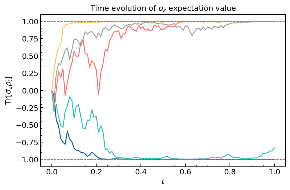
Projection onto \(\sigma_z\) eigenstate
expects_all = dq.expect(dq.sigmaz(), result.states).real

for expects in expects_all:
    plt.plot(tsave, expects, lw=1.5)

plt.axhline(-1, ls='--', lw=1.0, color='gray')
plt.axhline(1, ls='--', lw=1.0, color='gray')
plt.gca().set(
    title=r'Time evolution of $\sigma_z$ expectation value',
    xlabel=r'$t$',
    ylabel=r'$\langle \sigma_z \rangle_t=\langle \psi_t | \sigma_z | \psi_t \rangle$',
    ylim=(-1.1, 1.1),
)
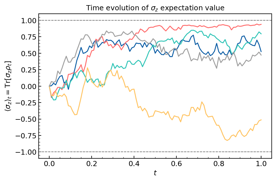
Imperfect detection
If the detection is imperfect, the system state is a density matrix. We use dq.dsmesolve() to simulate these quantum trajectories.
# define efficiencies
etas = [0.2]

# simulate trajectories
result = dq.dsmesolve(H, jump_ops, etas, psi0, tsave, keys, method=method)
print(result)
==== DSMESolveResult ====
Method       : EulerMaruyama
Infos        : 1000 steps | infos shape (5,)
States       : QArray complex64 (5, 101, 2, 2) | 7.9 Kb
Measurements : Array float32 (5, 1, 100) | 2.0 Kb
>>> result.states.shape  # (ntrajs, ntsave, n, n)
(5, 101, 2, 2)
>>> result.measurements.shape  # (ntrajs, nLm, ntsave-1)
(5, 1, 100)
expects_all = dq.expect(dq.sigmaz(), result.states).real

for expects in expects_all:
    plt.plot(tsave, expects, lw=1.5)

plt.axhline(-1, ls='--', lw=1.0, color='gray')
plt.axhline(1, ls='--', lw=1.0, color='gray')
plt.gca().set(
    title=r'Time evolution of $\sigma_z$ expectation value',
    xlabel=r'$t$',
    ylabel=r'$\langle \sigma_z \rangle_t = \mathrm{Tr}[\sigma_z\rho_t]$',
    ylim=(-1.1, 1.1),
)
Quantum harmonic oscillator
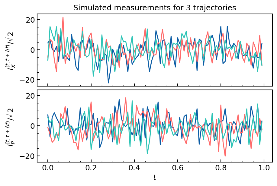
We consider a quantum harmonic oscillator starting from the coherent state \(\ket\alpha\), with Hamiltonian \(H=\omega a^\dagger a\) and a single loss operator \(L=\sqrt\kappa a\) which is continuously measured by heterodyne detection along the \(X\) and \(P\) quadratures with efficiency \(\eta\), resulting in two a diffusive measurement records \(I_X\) and \(I_P\). For this example the measurement backaction is null.
Simulation
# define Hamiltonian, jump operators, efficiencies, initial state
n = 16
a = dq.destroy(n)
kappa = 1.0
omega = 10.0
alpha0 = 2.0
H = omega * a.dag() @ a
jump_ops = [jnp.sqrt(kappa/2) * a, jnp.sqrt(kappa/2) * (-1j * a)]
etas = [1.0, 1.0]
psi0 = dq.coherent(n, alpha0)

# define save times
tsave = np.linspace(0, 1 / kappa, 101)
delta_t = tsave[1] - tsave[0]

# define a certain number of PRNG key, one for each trajectory
key = jax.random.PRNGKey(42)
ntrajs = 1000
keys = jax.random.split(key, ntrajs)

# simulate trajectories
method = dq.method.EulerMaruyama(dt=1e-3)
options = dq.Options(save_states=False)
result = dq.dsmesolve(H, jump_ops, etas, psi0, tsave, keys, method=method, options=options)
print(result)
==== SMESolveResult ====
Method       : Euler
Infos        : 1000 steps | infos shape (1000,)
States       : QArray complex64 (1000, 16, 16) | 2.0 Mb
Measurements : Array float32 (1000, 2, 100) | 781.2 Kb
>>> result.measurements.shape  # (ntrajs, nLm, ntsave-1)
(1000, 2, 100)
Individual trajectories
Iks_x = result.measurements[:, 0]
Iks_p = result.measurements[:, 1]
fig, axs = dq.plot.grid(2, 2, w=6, h=2, sharexy=True)
ax0, ax1 = list(axs)

for Ik_x in Iks_x[:3]:
    ax0.plot(tsave[:-1], Ik_x / np.sqrt(2), lw=1.5)

ax0.set(
    title=rf'Simulated measurements for 3 trajectories',
    ylabel=r'$I_X^{[t,t+\Delta t)}/\sqrt{2}$',
)

for Ik_p in Iks_p[:3]:
    ax1.plot(tsave[:-1], Ik_p / np.sqrt(2), lw=1.5)

ax1.set(
    xlabel=r'$t$',
    ylabel=r'$I_P^{[t,t+\Delta t)}/\sqrt{2}$',
)
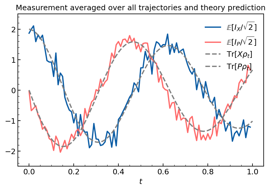
Averaged trajectories
plt.figure()
plt.plot(tsave[:-1], jnp.mean(Iks_x / np.sqrt(2), axis=0), label=r'$\mathbb{E}[I_X/\sqrt{2}]$')
plt.plot(tsave[:-1], jnp.mean(Iks_p / np.sqrt(2), axis=0), label=r'$\mathbb{E}[I_P/\sqrt{2}]$')

alpha = alpha0 * jnp.exp(-kappa / 2 * tsave) * jnp.exp(-1j * omega * tsave)
plt.plot(tsave, alpha.real, label=rf'$\mathrm{{Tr}}[X\rho_t]$', ls='--', color='gray')
plt.plot(tsave, alpha.imag, label=rf'$\mathrm{{Tr}}[P\rho_t]$', ls='--', color='gray')

plt.gca().set(
    title=r'Measurement averaged over all trajectories and theory prediction',
    xlabel=r'$t$',
    ylim=(-2.5, 2.5),
)
plt.legend()