Workflow in Dynamiqs
The core of Dynamiqs is to solve quantum differential equations. This tutorial goes over the basic workflow of such simulations, in mainly four steps:
- Define the system: Initialize the state and operators you are interested in.
- Set the scope: Specify the duration, observables to measure, or method to use.
- Run the simulation: Solve the differential equation and collect the results.
- Analyze the results: Plot results and extract the information you are interested in.
In the rest of this tutorial, we go over these steps in detail, taking the example of Rabi oscillations of a two-level system.
import dynamiqs as dq
import jax.numpy as jnp
import matplotlib.pyplot as plt

dq.plot.mplstyle(dpi=150)  # set custom matplotlib style
I. Define the system
After having imported the necessary packages, we can define our system, namely the initial state, the Hamiltonian, and the eventual loss operators. Common states and operators are already defined in Dynamiqs, see the Python API for more details. Otherwise, you can define specific states and operators using any array-like.
Here, we will use dq.fock() to define the initial state \(\ket{\psi_0}=\ket{0}\), dq.sigmaz() and dq.sigmax() to define the Hamiltonian \(H = \delta \sigma_z + \Omega \sigma_x\).
# initial state
psi0 = dq.fock(2, 0)

# Hamiltonian
delta = 0.3  # detuning
Omega = 1.0  # Rabi frequency
H = delta * dq.sigmaz() + Omega * dq.sigmax()

print(f"State of type {type(psi0)} and shape {psi0.shape}.")
print(f"Hamiltonian of type {type(H)} and shape {H.shape}.")
State of type <class 'dynamiqs.qarrays.dense_qarray.DenseQArray'> and shape (2, 1).
Hamiltonian of type <class 'dynamiqs.qarrays.sparsedia_qarray.SparseDIAQArray'> and shape (2, 2).
In Dynamiqs, all quantum objects are defined with the QArray type. All quantum objects have at least two dimensions to avoid systematic reshaping or coding mistakes (e.g. trying to multiply a ket and an operator in the wrong order). In particular, kets have shape (..., n, 1) and density matrices have shape (..., n, n).
II. Set the scope
Next, we define the scope of the simulation. This includes the total duration of time evolution, the observables we want to measure and how often we measure them. Observables are defined similarly to the Hamiltonian, using qarrays and Dynamiqs utility functions. The total duration and how often measurements are performed is defined in a single object named tsave. It is an arbitrary array of time points, of which tsave[-1] specifies the total duration of time evolution.
We also need to specify the method and options related to it, namely the method of integration and the eventual related parameters. The list of available methods and their parameters is available in the Python API.
# define sampling times
sim_time = 10.0  # total time of evolution
num_save = 101  # number of time slots to save
tsave = jnp.linspace(0.0, sim_time, num_save)  # can also be a list or a NumPy array

# define list of observables
exp_ops = [dq.sigmaz()]  # expectation value of sigma_z

# define method (Dormand-Prince method of order 5)
method = dq.method.Dopri5(rtol=1e-6, atol=1e-8)
III. Run the simulation
We can now run the simulation. This is done by calling the dq.sesolve() function, which returns an instance of SESolveResult. This object contains the computed states, the observables, and various information about the method.
# run simulation
result = dq.sesolve(H, psi0, tsave, exp_ops=exp_ops, method=method)

# print some information
print(f"`result` is of type {type(result)}.")
print(f"`result` has the following attributes:")
print(f"{[attr for attr in dir(result) if not attr.startswith('__')]}\n")
print(result)
`result` is of type <class 'dynamiqs.result.SESolveResult'>.
`result` has the following attributes:
['_abc_impl', '_saved', '_str_parts', 'block_until_ready', 'expects', 'extra', 'final_state', 'gradient', 'infos', 'method', 'options', 'states', 'to_numpy', 'to_qutip', 'tsave']

|██████████| 100.0% ◆ elapsed 4.57ms ◆ remaining 0.00ms
==== SESolveResult ====
Method  : Dopri5
Infos   : 56 steps (48 accepted, 8 rejected)
States  : QArray complex64 (101, 2, 1) | 1.6 Kb
Expects : Array complex64 (1, 101) | 0.8 Kb
IV. Analyze the results
Finally, you can analyze the results in whichever way is most relevant to your application. In our example, let us plot the \(\braket{\sigma_z}\) observable as a function of time. To do so, we call result.expects[0].real which extracts the first measured observable (here, the only one) and plot its real part (our observable is hermitian, so measurements are real-valued). We compare to the expected analytical result.
# analytical result
Omega_star = jnp.sqrt(delta**2 + Omega**2)  # generalized Rabi frequency
excited_pop = Omega / Omega_star * jnp.sin(tsave * Omega_star)  # excited population
sigmaz_analytical = 1 - 2 * excited_pop**2  # expectation value of sigma_z

# plot results
plt.plot(tsave, sigmaz_analytical, 'k', lw=1.0)
plt.plot(tsave, result.expects[0].real, 'oC0', ms=4)

# formatting
plt.xlabel('Time')
plt.ylabel(r'$\langle \sigma_z \rangle$')
plt.xlim(0, 10)
plt.ylim(-1, 1)
plt.legend(('Analytical', 'Dynamiqs'))
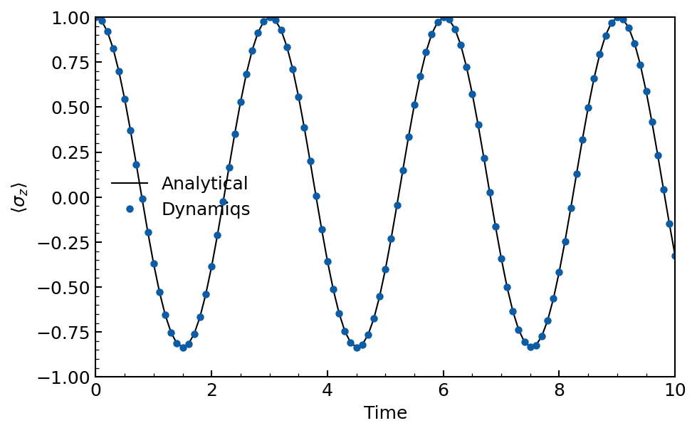
As expected, we find off-resonant Rabi oscillations at the generalized Rabi frequency \(\Omega^* = \sqrt{\delta^2 + \Omega^2}\), and with a reduced amplitude \(|\Omega / \Omega^*|^2\).