Driven-dissipative Kerr oscillator
In this example, we show how to simulate a driven-dissipative Kerr oscillator in Dynamiqs. It is a simple example of a non-linear quantum harmonic oscillator with dissipative coupling to its environment. In the appropriate rotating frame, it is described by the master equation $$ \frac{\dd\rho}{\dt} = -i [H(t), \rho] + \kappa \mathcal{D}[a] (\rho), $$ with Hamiltonian $$ H(t) = -K a^{\dagger 2} a^2 + \epsilon(t) a^\dagger + \epsilon^*(t) a, $$ with \(\kappa\) the rate of single-photon dissipation, \(K\) the Kerr non-linearity, and \(\epsilon(t)\) the driving field.
import dynamiqs as dq
import jax
import jax.numpy as jnp
import matplotlib.pyplot as plt

dq.plot.mplstyle(dpi=150)  # set custom matplotlib style
Basic time evolution
Let us begin with a simple simulation of the time evolution of this system, assuming that the driving field is constant and the system is initially in a coherent state.
# simulation parameters
n = 32         # Hilbert space size
K = 1.0        # Kerr non-linearity
epsilon = 3.0  # driving field
kappa = 1.5    # dissipation rate
alpha0 = 2.0   # initial coherent state amplitude
T = 5.0        # simulation time
ntsave = 201   # number of saved states

# operators
a = dq.destroy(n)
H = -K * a.dag() @ a.dag() @ a @ a + epsilon * (a + a.dag())
jump_ops = [jnp.sqrt(kappa) * a]

# initial state
psi0 = dq.coherent(n, alpha0)

# save times
tsave = jnp.linspace(0.0, T, ntsave)

# run simulation
result = dq.mesolve(H, jump_ops, psi0, tsave)
From this simulation, we can extract any property of the evolved state at any saved time. We can for instance access the number of photons in the final state using
>>> dq.expect(a.dag() @ a, result.states[-1])
Array(1.434+0.j, dtype=complex64)
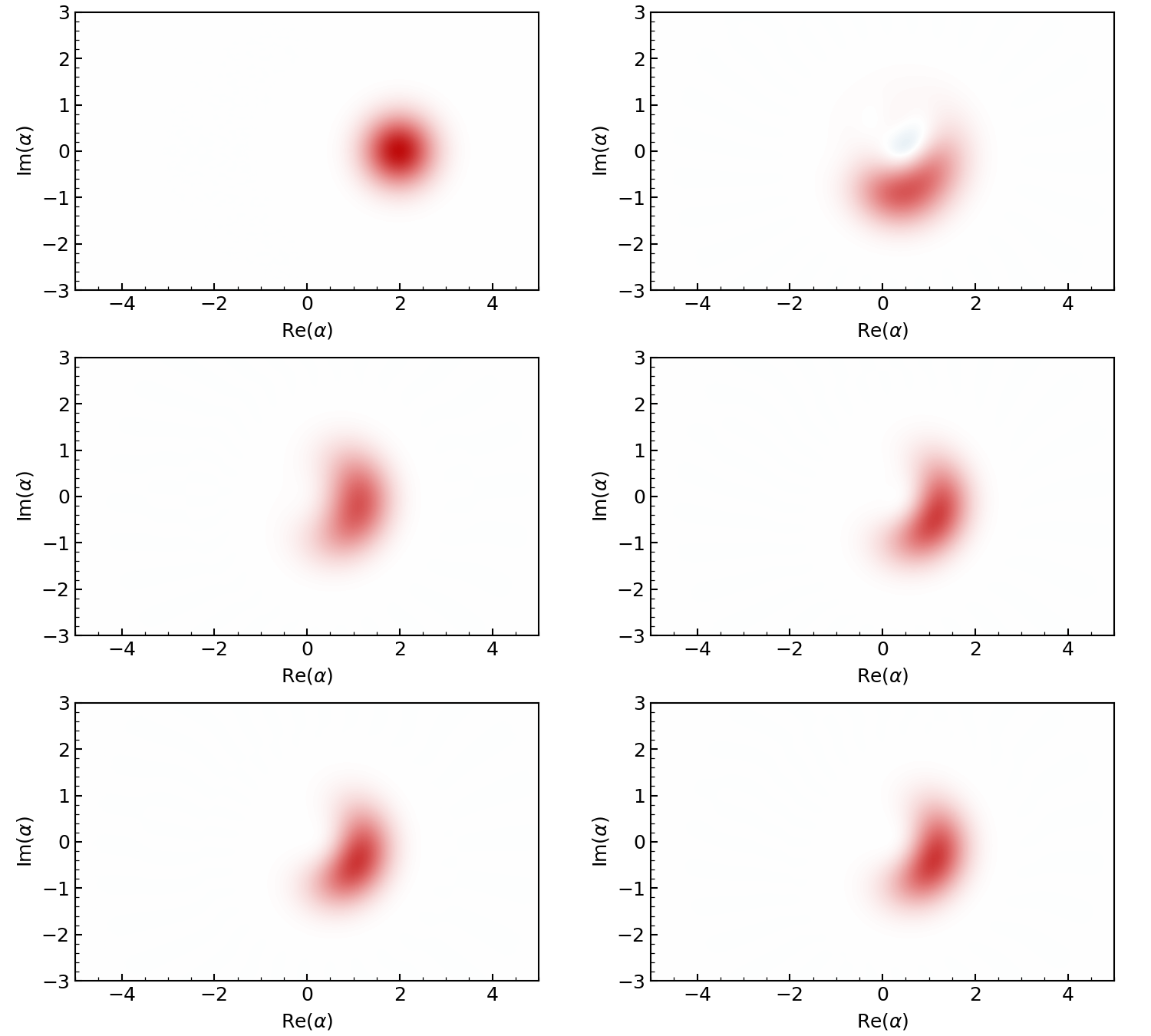
Alternatively, we can also plot the Wigner function of the evolved state.
gif = dq.plot.wigner_gif(result.states, ymax=3.0, gif_duration=10.0)
Periodic revival of a coherent state
Time evolution of the cavity field
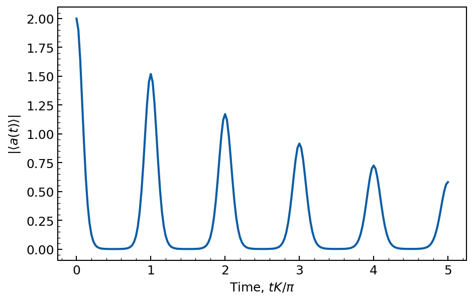
One of the most striking features of the Kerr oscillator is the periodic revival of the initial coherent state. This phenomenon is a direct consequence of the non-linear interaction between the photons in the cavity. We can observe this effect by plotting the absolute value of the cavity field as a function of time, for a simulation time over several units of Kerr, and as long as photon loss is not too important.
# simulation parameters
n = 32
K = 1.0
kappa = 0.02
alpha0 = 2.0
ntsave = 201

# operators
a = dq.destroy(n)
H = -K * a.dag() @ a.dag() @ a @ a
jump_ops = [jnp.sqrt(kappa) * a]

# initial state
psi0 = dq.coherent(n, alpha0)

# save times
T = 5 * jnp.pi / K
tsave = jnp.linspace(0.0, T, ntsave)

# expectation operator
exp_ops = [a]

# run simulation
result = dq.mesolve(H, jump_ops, psi0, tsave, exp_ops=exp_ops)

# plot cavity field
plt.plot(tsave * K / jnp.pi, jnp.abs(result.expects[0]))
plt.xlabel(r'Time, $tK / \pi$')
plt.ylabel(r'$|\langle a(t) \rangle|$')
We indeed observe a periodic revival of the coherent state, with a period of \(\pi / K\). These revivals have a reduced amplitude due to the presence of photon loss.
Study of revivals
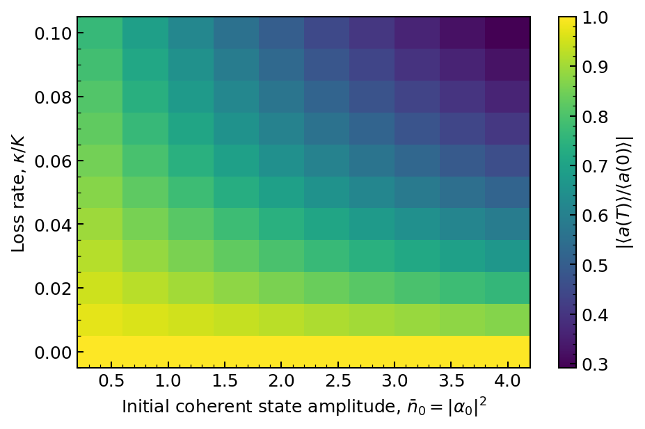
We can further investigate these periodic revivals by plotting the amplitude of the first revival as a function of the photon loss \(\kappa\), and as a function of the initial coherent state amplitude. To do so, we make use of a powerful feature of Dynamiqs: the ability to batch simulations concurrently. Here, we can batch over both a jump operator and the initial state.
# parameters to sweep
kappas = jnp.linspace(0.0, 0.1, 11)
nbar0s = jnp.linspace(0.4, 4.0, 10)
alpha0s = jnp.sqrt(nbar0s)

# redefine jump operators and initial states
jump_ops = [jnp.sqrt(kappas[:, None, None]) * a] # using numpy broadcasting
psi0 = dq.coherent(n, alpha0s) # dq.coherent accepts a batched input

# save times
T = jnp.pi / K  # a single revival
tsave = jnp.linspace(0.0, T, 100)

# run batched simulation
result = dq.mesolve(H, jump_ops, psi0, tsave, exp_ops=exp_ops)
amp_revivals = jnp.abs(result.expects[:, :, 0, -1] / result.expects[:, :, 0, 0])

# plot a 2D map of the normalized amplitude revivals
contour = plt.pcolormesh(nbar0s, kappas / K, amp_revivals)
cbar = plt.colorbar(contour, label=r'$|\langle a(T) \rangle / \langle a(0) \rangle |$')
plt.xlabel(r'Initial coherent state amplitude, $\bar{n}_0 = |\alpha_0|^2$')
plt.ylabel(r'Loss rate, $\kappa / K$')
We observe that the amplitude of the first revival decreases monotically with the photon loss rate \(\kappa\), and with the initial coherent state amplitude \(\bar{n}\). This behavior is consistent with the expected behavior of the Kerr oscillator. Remarkably, thanks to batching, such a set of hundreds of simulations can be run in a few seconds.
The transmon regime
In this section, we investigate the driven-dissipative Kerr oscillator in the transmon regime, where the Kerr non-linearity is much larger than the driving field and the dissipation rate, \(K \gg |\epsilon| \gg \kappa\). In this regime, the two lowest-energy Fock states are frequency-detuned and thus decoupled from the rest of the system, allowing for quantum information processing.
Rabi oscillations
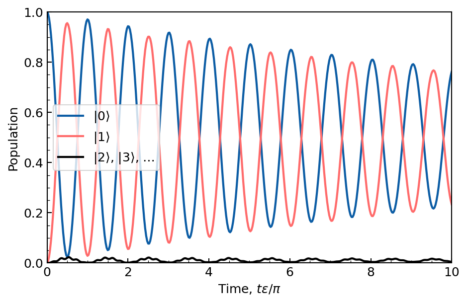
Because this regime describes an effective two-level system, we can observe Rabi oscillations. These can be simulated by constant driving the system initialized in vacuum.
# simulation parameters
n = 8
K = 200.0
epsilon = 40.0
kappa = 1.0
T = 10 * jnp.pi / epsilon
ntsave = 401

# operators
a = dq.destroy(n)
H = -K * a.dag() @ a.dag() @ a @ a + epsilon * (a + a.dag())
jump_ops = [jnp.sqrt(kappa) * a]

# initial state
psi0 = dq.basis(n, 0)

# save times
tsave = jnp.linspace(0.0, T, ntsave)

# expectation operator
exp_ops = [dq.proj(dq.basis(n, 0)), dq.proj(dq.basis(n, 1))]

# run simulation and extract observables
result = dq.mesolve(H, jump_ops, psi0, tsave, exp_ops=exp_ops)
pop_0 = result.expects[0].real # population of |0>
pop_1 = result.expects[1].real # population of |1>

# plot Rabi oscillations
plt.plot(tsave * epsilon / jnp.pi, pop_0, label=r'$|0\rangle$')
plt.plot(tsave * epsilon / jnp.pi, pop_1, label=r'$|1\rangle$')
plt.plot(tsave * epsilon / jnp.pi, 1 - (pop_0 + pop_1), color='black', label=r'$|2\rangle$, $|3\rangle$, $\ldots$')
plt.xlabel(r'Time, $t\epsilon / \pi$')
plt.ylabel('Population')
plt.ylim(0, 1)
plt.xlim(0, T * epsilon / jnp.pi)
plt.legend(frameon=True)
We indeed find Rabi oscillations between Fock states \(|0\rangle\) and \(|1\rangle\), with a period of \(\pi / \epsilon\). However, these oscillations are damped due to the presence of photon loss. In addition, we observe that a small fraction of the total population is periodically leaked to higher Fock states. This is because the Kerr oscillator is not a perfect two-level system, and the driving field is too large compared to the Kerr non-linearity.
A gaussian pi-pulse
We now study the optimization of a single-qubit gate for this effective two-level system, a crucial step in quantum information processing. More precisely, we aim to find the best parameters to maximize the fidelity of a \(\pi\)-pulse, i.e., a pulse that swaps the populations of the two lowest-energy Fock states. To do so, we need to balance the amplitude damping due to photon loss with the leakage to higher excited states due to finite pulse duration.
We define a pulse ansatz and optimize the \(\pi\)-pulse fidelity by sweeping the parameters of this ansatz. The ansatz we study is that of a truncated gaussian, of the form
where \(T\) the gate duration, and \(\sigma\) the normalized pulse width. One can easily check that the pulse area condition is satisfied, i.e.,
We begin by defining the pulse ansatz:
from jax.scipy.special import erf

def pulse(t, T, sigma):
    """Gaussian pulse ansatz."""
    angle = jnp.pi / 2
    norm = jnp.sqrt(2 * jnp.pi) * sigma * T * erf(1 / (2 * jnp.sqrt(2) * sigma))
    gaussian = jnp.exp(-(t - T / 2)**2 / (2 * T**2 * sigma**2))
    return angle * gaussian / norm
Then, we can define our sweeping parameters, and run the simulation by combining batching over dq.modulated to batch over the pulse width, and a jax.vmap to batch over the gate duration.
from functools import partial

# simulation parameters
n = 8
K = 200.0
kappa = 1.0
ntsave = 401

# parameters to sweep
Ts = jnp.linspace(0.05, 0.5, 24)
sigmas = jnp.linspace(0.05, 0.2, 14)

# operators, initial state, and expectation operator
a = dq.destroy(n)
H0 = -K * a.dag() @ a.dag() @ a @ a
jump_ops = [jnp.sqrt(kappa) * a]
psi0 = dq.basis(n, 0)
exp_ops = [dq.proj(dq.basis(n, 0)), dq.proj(dq.basis(n, 1))]

@jax.vmap
def compute_fidelity(T):
    """Compute the fidelity of a pi-pulse for a given gate duration."""
    # time-dependent Hamiltonian, defined with functools.partial and broadcasting
    # `f` has signature (t: float) -> Array of shape (len(sigmas),)
    f = partial(pulse, T=T, sigma=sigmas)
    H = H0 + dq.modulated(f, a + a.dag())

    # save times
    tsave = jnp.linspace(0.0, T, ntsave)

    # run simulation
    result = dq.mesolve(H, jump_ops, psi0, tsave, exp_ops=exp_ops)

    # fidelity is roughly estimated as the largest overlap with |1>
    # in a proper study, we would need to compute a full process tomography
    return jnp.max(result.expects[:, 1, :].real, axis=-1)

# run simulation
fidelities = compute_fidelity(Ts)

# plot results
plt.pcolormesh(sigmas, Ts, jnp.log10(1-fidelities), cmap='Blues_r')
plt.xlabel('Pulse width')
plt.ylabel('Gate duration')
plt.colorbar(label='log10(1 - Fidelity)')
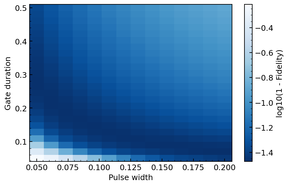
We observe that the fidelity of the \(\pi\)-pulse is maximized over a band of pulse widths and gate durations. In practice, one wants to reduce the gate duration as much as possible, but this corresponds to large pulse widths. However, such large-width truncated gaussians are not physical because they do not verify \(\epsilon(0) = \epsilon(T) = 0\), and similarly for higher derivatives. This is a limitation of our gaussian ansatz, and one would need to consider more complex pulse shapes to optimize this \(\pi\)-pulse in a realistic setting.
Optimization with GRAPE
In this section, we turn to the numerical optimization of the \(\pi\)-pulse using gradient ascent pulse engineering (GRAPE). This method consists of parametrizing the input pulse through a piece-wise constant function, and optimizing each parameter through gradient descent.
To do so, we use the optax library for optimization, which provides a simple interface to various gradient descent algorithms. We define a loss function to minimize, which is the negative fidelity of the \(\pi\)-pulse, and a smoothness loss to penalize sharp variations in the pulse. We then run the optimization loop.
import optax

# simulation parameters
n = 8
K = 200.0
kappa = 1.0
T = 0.2
ntsave = 401

# optimization parameters
ntpulse = 101       # number of pieces in the parametrized pulse
nepochs = 300       # number of optimization epochs
learning_rate = 0.2 # gradient descent learning rate

# operators, initial state, and expectation operator
a = dq.destroy(n)
H0 = -K * a.dag() @ a.dag() @ a @ a
jump_ops = [jnp.sqrt(kappa) * a]
psi0 = dq.basis(n, 0)
exp_ops = [dq.proj(dq.basis(n, 0)), dq.proj(dq.basis(n, 1))]

# save times and pulse times (not necessarely the same)
tsave = jnp.linspace(0.0, T, ntsave)
tpulse = jnp.linspace(0.0, T, ntpulse)

# function to optimize
def compute_fidelity(amps):
    # time-dependent Hamiltonian
    # (sum of two piece-wise constant Hamiltonians and of the static Hamiltonian)
    Hx = dq.pwc(tpulse, jnp.real(amps), a + a.dag())
    Hp = dq.pwc(tpulse, jnp.imag(amps), 1j * (a - a.dag()))
    H = H0 + Hx + Hp

    # run simulation
    options = dq.Options(progress_meter=False) # disable progress meter
    result = dq.mesolve(H, jump_ops, psi0, tsave, exp_ops=exp_ops, options=options)

    # fidelity is now defined as the overlap with |1> at the final time only
    return result.expects[1, -1].real

# losses to minimize
@jax.jit
def compute_fidelity_loss(amps, weight=1.0):
    return weight * (1 - compute_fidelity(amps))

@jax.jit
def compute_smoothness_loss(amps, weight=1e-4):
    return weight * jnp.sum(jnp.abs(jnp.diff(jnp.pad(amps, 1)))**2)

# seed amplitudes
amps_seed = 0.5 * jnp.pi / T * jnp.ones(ntpulse - 1) + 1j * jnp.zeros(ntpulse - 1)

# optimization loop
optimizer = optax.adam(learning_rate)
amps = amps_seed
opt_state = optimizer.init(amps)
losses = []
for _ in range(nepochs):
    # compute losses and their gradients with `jax.value_and_grad`
    fidelity_loss, fidelity_grad = jax.value_and_grad(compute_fidelity_loss)(amps)
    smoothness_loss, smoothness_grad = jax.value_and_grad(compute_smoothness_loss)(amps)
    grads = fidelity_grad + smoothness_grad

    # update amplitudes with optimizer
    updates, opt_state = optimizer.update(grads.conj(), opt_state)
    amps = optax.apply_updates(amps, updates)

    # store losses
    losses.append([fidelity_loss, smoothness_loss])

# plot optimized pulse
dq.plot.pwc_pulse(tpulse, amps)
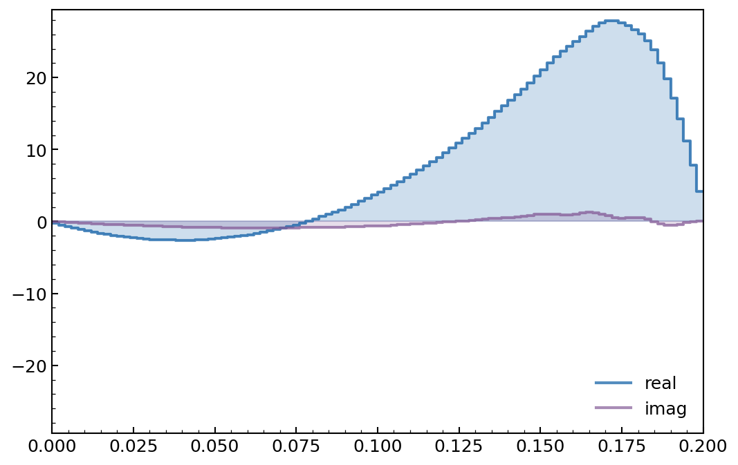
We indeed find a smooth pulse, with a small contribution on the imaginary part corresponding to a drive on the conjugate quadrature. This is typical of an optimal transmon pulse, in which leakage is minimized through this additional drive in a process known as Derivative Removal by Adiabatic Gate (DRAG).
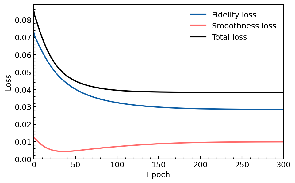
We can also plot the evolution of the fidelity and smoothness losses during the optimization process.
losses = jnp.asarray(losses)
plt.plot(losses[:, 0], label="Fidelity loss")
plt.plot(losses[:, 1], label="Smoothness loss")
plt.plot(losses[:, 0] + losses[:, 1], c='k', label="Total loss")
plt.ylim(0)
plt.xlim(0, nepochs)
plt.ylabel("Loss")
plt.xlabel("Epoch")
plt.legend()
We find that the overall loss decreases monotonically, with a smoothness loss kept relatively low compared to the fidelity loss. We also find convergence of the loss function, indicating that the optimization process is successful. Of course, the hyper parameters such as the relative weight of each loss, the number of pulse time steps, the learning rate, or the number of epochs, could be further tuned.
For optimal control applications, we also recommend checking out qontrol which is build on top of Dynamiqs, and provides a more advanced interface for pulse optimization.
